Step by Step Derivation of the Propagator
1 The Approach
The first part of QFT is a free particle theory (no interactions, see Unifying Chart 3, Part 1). After this, interactions are introduced (U.C. 3, Part 2). In the course of deriving the interaction theory, a mathematical relationship arises that is called the Feynman propagator. Physically, it can be visualized as representing a virtual particle that exists fleetingly and carries energy, momentum, and in some cases, charge from one real particle to another. Thus, it is the carrier or mediator of force (interaction.)
Heuristically, it may help to consider the virtual
particle as created at a particular spacetime point and destroyed at a later
spacetime point, and this is how Feynman diagrams portray it. From this (heuristic) perspective the field
operator † (y) can
be considered to create a virtual scalar particle at y, and the field
operator
(x) destroys that virtual particle at x. The scalar propagator incorporates these two
field operators in a sort of “short-hand” way.
Note that the above “creation/destruction at a point” perspective can help initially in understanding the derivation of the propagator, but we caution that it will have to be modified and refined. We will save that to the end when, after digesting the derivation to follow, this modification will be easier to understand.
We will now derive a relationship for the propagator using the field operators acting on the vacuum, and will later see (U.C. 3, Part 2) that this derived relationship arises naturally in the full mathematical development of the interaction theory.
2 Milestones in the Derivation
We start with the coefficient commutation relations and
proceed in five distinct steps. The
entire derivation is for continuous (rather than discrete) eigenstate solutions
of the field equation (Klein-Gordon here), since the propagator represents a
virtual particle in the vacuum and the vacuum is unbounded. We represent the scalar Feynman propagator
with the symbol .
As noted, our starting point is the coefficient commutators
|
|
and from there we follow five steps. The first two are purely mathematical, and will serve as background that will help us with the remaining steps. The third step comprises a physical interpretation of the propagator, and the last two steps are mathematical manipulations to get that interpretation into convenient form (the form that is used in QFT interaction analysis.)
1.
First Step: Use (1)
to find commutation relations for positive and negative frequency solutions,
i.e., determine what is in
|
|
where Δ± is different from the
propagator ΔF, and (2)
is found in terms of an integral over 3 momentum k (as the ± (x) and
† ± (y)
are integrals over 3-momentum).
3. Third Step: Express the Feynman propagator ΔF as a time ordered operator (actually the vacuum expectation value of this operator), which represents a particle or antiparticle created at one point in space and time in the vacuum and destroyed at another place and time.
4. Fourth Step: Express ΔF as a contour integral in the space of 4-momenta (with the help of the second step above.)
5. Fifth Step: Re-express ΔF as an integral over real (rather than complex) energy and 3-momenta. This is the form most suitable for analysis.
3 The Derivation
3.1 Step 1: Commutation Relations for Positive/Negative Frequency Solutions
Define
|
|
(3) |
Then, substituting the integral (boundary free, continuous) form for the Klein-Gordon solutions gives
|
|
(4) |
and thus,
|
|
Similarly,
|
|
(6) |
leads to
|
|
3.2 Step 2: Expressing iΔ± as Contour Integrals
 Consider
the complex plane for a function f of the complex variable k0, i.e., f (k0). Here, the symbol k0 is not a pole (poles are usually designated with null
subscript), but represents a complex number generalization of the zeroth
component (the energy) of 4-momentum k.
We concern ourselves with the particular case where k0 takes on the
real value ωk. From complex variable theory,
Consider
the complex plane for a function f of the complex variable k0, i.e., f (k0). Here, the symbol k0 is not a pole (poles are usually designated with null
subscript), but represents a complex number generalization of the zeroth
component (the energy) of 4-momentum k.
We concern ourselves with the particular case where k0 takes on the
real value ωk. From complex variable theory,
|
|
Now, re-express (5) as
|
|
where we take the bracketed quantity as equal to f (ωk), and where
|
|
We can then use (10) in (8) to re-express f (ωk) in terms of a contour integral. Using this for the bracket in (9), we find (9) becomes
|
|
where the integral notation now
implies integration over four dimensions of the 4-momentum, with the 3-momentum
part from ∞ to +∞ in real space and the energy part a
contour integral in complex space. Note
that the integral does not “blow up” because k0 ≠ ωk over the contour integral. We are using a mathematical trick that
works, though it jars our usual understanding that, for real particles, the
zeroth component of 4-momentum equals energy.
k0 has
at this point become, for us, a variable that generally does not equal energy ωk.
We modify (11) a little by noting what is always true mathematically for any four vector, and thus true for 4-momentum components,
|
|
and what is physically true for rest mass, energy, and 3-momentum,
|
|
Solve these last two relations for k0 and ωk and substitute in the last line of (11) to get
|
|
 For iΔ
(x
y), we carry out similar steps except
that the contour integral (still c.c.w.) is now about
ωk.
When all is said and done, we find the only difference from (14)
to be the contour, which is now about the negative frequency value and designed
by C
.
|
|
3.3 Step 3: The Feynman Propagator as the VEV of a Time Order Operator
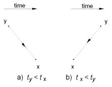 Figure
3a) represents creation of a particle, which will be virtual, at y and
destruction of it at x. Figure
3b) represents creation of an antiparticle at x and destruction of it at
y. Virtual particles are never
detected when real particles interact, so the same effect on the real particles
could be realized by either of the processes in Figure 3. For example, a virtual particle carrying
charge from y to x would represent the same charge exchanges as
an antiparticle carrying opposite charge from x to y. Thus, we need a relationship for the
propagator that includes both scenarios as possibilities.
Figure
3a) represents creation of a particle, which will be virtual, at y and
destruction of it at x. Figure
3b) represents creation of an antiparticle at x and destruction of it at
y. Virtual particles are never
detected when real particles interact, so the same effect on the real particles
could be realized by either of the processes in Figure 3. For example, a virtual particle carrying
charge from y to x would represent the same charge exchanges as
an antiparticle carrying opposite charge from x to y. Thus, we need a relationship for the
propagator that includes both scenarios as possibilities.
To this end, we need an operator that will create a particle first if ty < tx, but create an antiparticle first if tx < ty. Consider the time ordered operator T, defined as follows.
If ty
< tx, † (y)
operates first (creates a particle) and is placed on the right, with
(x) operating second
(destroys the particle) and placed on the left.
|
|
(16) |
If tx < ty, (x) operates first (creates
an antiparticle) and is placed on the right with
† (y)
operating second (destroying the antiparticle) and placed on the left.
|
|
(17) |
We now define what is called the transition amplitude density, which equals the vacuum expectation value (VEV) of the above time ordered operator. It is an amplitude, similar to the amplitude of a wave function in NRQM, because, as we will shortly see, the square of its magnitude equals the probability density of it being observed. (As the square of the magnitude of the amplitude for a component of the wave function equals the probability of it being observed.)
This transition amplitude density is
|
|
and this represents both possible scenarios of Figure 3. In wave mechanics, the bracket above is an integration over all space. This is still true, but note carefully that the integration variable is over the space variable of the bra and ket (think x′), but not the time ordered variables x and y. In matrix mechanics, we merely think of a bracket as equaling zero unless the bra and ket represent the same particle(s).
To gain insight into (18), consider the transition amplitude density operating on the vacuum when a virtual particle is propagated. Then,
|
|
where G, F, and H
are numeric factors that result from the creation and destruction operations
(such as the normalization coefficients that are part of the field operators),
which we will not express explicitly here.
Thus, we have a general ket left, which in this case is part vacuum
state, with the amplitude of the vacuum state part being GF, and the
amplitude of the multiparticle state (scalar plus anti-scalar) part being HF. For appropriate normalization, the square of
the magnitude of GF is the probability of observing the vacuum (no
particles left after the transition.)
To find the amplitude GF, we need only form an inner product of
the last line of (19)
with 0
,
i.e.,
|
|
(20) |
Thus, the VEV of the time ordered operator is an amplitude, the square of whose magnitude is the probability of the transition from vacuum initially to vacuum finally. Actually, |G(x)F(y)|2 is a probability density (to be precise, a double density), because it is a function of x and y. We would need to integrate this over all x and y to get the actual probability, and this is what one does in interaction theory to calculate probabilities and cross sections.
In a similar way, the same time ordered operator can be used for antiparticle propagation (with time for x and y reversed.)
Given all of this, we can define the Feynman propagator ΔF (where the factor of i is introduced with foresight) by
|
|
3.4 Expressing ΔF as a Contour Integral
For ty < tx,
|
|
(22) |
where the last line follows from
the prior one because Δ+(x y) is numeric and includes no operators.
For tx < ty, in similar fashion, we find
|
|
(23) |
In summary,
|
|
where in section 3.2, we expressed Δ±(x y) as contour integrals, and thus we have
here expressed the Feynman propagator in terms of contour integrals. Note also, that the Feynman propagator,
although encompassing operators in its initial definition, turns out to be
simply a numeric quantity without operators.
3.5 Step 5: Re-express ΔF in Most Convenient Form
We would like two things more: 1) express the propagator
as a single function so we don’t have to keep track (while we are integrating
over spacetime and doing other things) of whether the virtual field is a
particle or antiparticle (i.e., whether to use the Δ+ or Δ function), and 2) have all our integrations
over real numbers rather than deal with contour integrals.
To do this, consider Figure 4 where we have shown two
contour integrals. The top loop
represents Δ and encloses
ωk with a ccw path. The lower loop encloses +ωk, but since it has a cw
integration path, represents
Δ+.
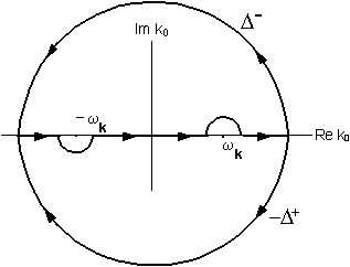
Thus, we can define the Feynman propagator of (24) as
ΔF
(integral of Fig 4 for either loop),
where the proportionality sign takes care of the concomitant integration over k, as well as the various constants involved.
 So
we can then re-write the propagator (24) with
(14),
(15),
and Figure 4 as
So
we can then re-write the propagator (24) with
(14),
(15),
and Figure 4 as
|
|
where the CF on the integral defines the route we take in the plane of Figure 4.
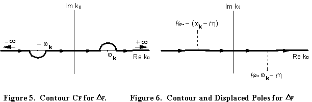
Now, consider enlarging the outer hemispheric parts of the two loops in Figure
4 so they extend essentially to infinity.
The value of the contour integrals over them will remain unchanged. But the k2 value in the denominator of (25)
will become so large that any contribution to the integral over those parts of
the path will become negligible. This
means that we can effectively take the integral of (25) as
extending only along the real axis from minus to plus infinity as in Figure 5.
We can further simplify by moving the poles an infinitesimal distance η off the real axis as shown in Figure 6 and deform the contour so that it is all along the real axis. In the limit as η → 0, the integral will have the same value, though we must now include this slight pole shift in the propagator expression (25). We do this by recalling from (12) and (13) that we used
|
|
to obtain the denominator of (25), so we must temporarily restate (25) using the right hand side of (26), then shift the poles. Thus, (25) becomes
|
|
(27) |
If we then use (26) again, ignore second order terms in η, and take ε = 2ηωk, we have our final result for the Feynman scalar propagator
|
|
Note the advantages of this form. We now have a single mathematical relationship that automatically describes both a particle propagating from y to x and an antiparticle propagating from x to y. We also have done away with the cumbersome contour integrals in favor of a simple 4D integral over the entire 4-momentum space. In practice, we can evaluate this integral then take ε to zero after the integration is carried out.
4 Comments on the Propagator and Its Derivation
4.1 The Propagator and Interaction Theory
The derivation above was formulated with an eye to interaction theory. In that theory, amplitudes are derived for various kinds of interactions between various particles. The square of the magnitude of each amplitude turns out to be the probability of that particular interaction (transition) occurring. These transition amplitudes each depend on the initial real particles, the final real particles, and the virtual particle(s) that mediate the transition. It turns out that the factor in the amplitude representing the virtual particle contribution is identical to the Feynman propagator ΔF as we defined it in the VEV of the time ordered operator (21). Thus, it is also equal to (28), so we can simply plug the RHS of (28) into the overall transition amplitude as part of our analysis.
This is one reason we started with the relation †
to create and destroy a virtual scalar particle, rather than what one might
initially expect, the simpler creation and destruction operator relation a(k)a†(k). Our heuristic approach was tailored to match
what we knew would be coming in the mathematical development of interaction
theory.
4.2 Meaning of Spacetime Points y and x
In Figure 3a we imply the virtual particle is created at y and destroyed at x. In Feynman diagrams virtual particles are depicted in this way, and the real incoming particle can be thought of a being destroyed at y, often with an outgoing real particle created at y. The virtual particle is also thus created at y. At x the virtual is destroyed, with the simultaneous creation of at least one outgoing real particle at x, often accompanied by the destruction of another real incoming particle at x.
To be precise, it is more correct to think of the incoming, outgoing, and virtual particles as moving waves spread out in space. What we calculate for a given y and x is the probability density for the interaction as a function of the coordinates y and x. If y and x are closer the probability density for the interaction to occur is greater; if farther away, the probability density is less. Integrating over all x and y gives the total probability for observing the interaction.
4.3 Momentum Space Form of the Propagator
From (28), we can readily write down the 4-momentum space form of the propagator, which will be very useful,
|
|
(29) |
4.4 Spinor and Vector Propagators
In parallel fashion to all of the above, we can derive Feynman propagators for Dirac particles and photons.
For spin particles,
|
|
(30) |
|
|
(31) |
For photons,
|
|
(32) |
|
|
(33) |
-
Links:
Unifying Chart 3, Part 1 (From Field Eqs to Propagators and Observables)
Unifying Chart 3, Part 2 (Interaction Theory. From Operators and Propagators to Feynman rules.)